캐글(Kaggle)의 "Bag of Words meets bag of popcorns"
(https://www.kaggle.com/c/word2vec-nlp-tutorial)
워드팝콘 데이터의 처리 과정
케글 데이터 불러오기 -> EDA -> 데이터정제 -> 모델링
데이터정제
- HTML 및 문장 보호 제거
- 불용어 제거
- 단어 최대 길이 설정
- 단어 패딩
- 백터 표상화
import zipfileDATA_IN_PATH = './data_in/'file_list = ['labeledTrainData.tsv.zip', 'unlabeledTrainData.tsv.zip', 'testData.tsv.zip']
file_list_tsv = ['labeledTrainData.tsv', 'unlabeledTrainData.tsv', 'testData.tsv']! ls ./data_inNanumGothic.ttf ratings.txt test_id.npy
labeledTrainData.tsv ratings_test.txt train_clean.csv
labeledTrainData.tsv.zip ratings_train.txt train_input.npy
nsmc_test_input.npy sampleSubmission.csv train_label.npy
nsmc_test_label.npy testData.tsv unlabeledTrainData.tsv
nsmc_train_input.npy testData.tsv.zip unlabeledTrainData.tsv.zip
nsmc_train_label.npy test_clean.csv
# file_list의 zip 압축파일을 풀어준다.
for file in file_list:
    zipRef = zipfile.ZipFile(DATA_IN_PATH + file, 'r')
    zipRef.extractall(DATA_IN_PATH)
    zipRef.close()
import numpy as np
import pandas as pd
import os
import matplotlib.pyplot as plt
import seaborn as sns
%matplotlib inline! head -2 ./data_in/labeledTrainData.tsvid sentiment review
"5814_8" 1 "With all this stuff going down at the moment with MJ i've started listening to his music, watching the odd documentary here and there, watched The Wiz and watched Moonwalker again. Maybe i just want to get a certain insight into this guy who i thought was really cool in the eighties just to maybe make up my mind whether he is guilty or innocent. Moonwalker is part biography, part feature film which i remember going to see at the cinema when it was originally released. Some of it has subtle messages about MJ's feeling towards the press and also the obvious message of drugs are bad m'kay.
Visually impressive but of course this is all about Michael Jackson so unless you remotely like MJ in anyway then you are going to hate this and find it boring. Some may call MJ an egotist for consenting to the making of this movie BUT MJ and most of his fans would say that he made it for the fans which if true is really nice of him.
The actual feature film bit when it finally starts is only on for 20 minutes or so excluding the Smooth Criminal sequence and Joe Pesci is convincing as a psychopathic all powerful drug lord. Why he wants MJ dead so bad is beyond me. Because MJ overheard his plans? Nah, Joe Pesci's character ranted that he wanted people to know it is he who is supplying drugs etc so i dunno, maybe he just hates MJ's music.
Lots of cool things in this like MJ turning into a car and a robot and the whole Speed Demon sequence. Also, the director must have had the patience of a saint when it came to filming the kiddy Bad sequence as usually directors hate working with one kid let alone a whole bunch of them performing a complex dance scene.
Bottom line, this movie is for people who like MJ on one level or another (which i think is most people). If not, then stay away. It does try and give off a wholesome message and ironically MJ's bestest buddy in this movie is a girl! Michael Jackson is truly one of the most talented people ever to grace this planet but is he guilty? Well, with all the attention i've gave this subject....hmmm well i don't know because people can be different behind closed doors, i know this for a fact. He is either an extremely nice but stupid guy or one of the most sickest liars. I hope he is not the latter."
# 데이터를 불러오자
train_data = pd.read_csv(DATA_IN_PATH + 'labeledTrainData.tsv', header=0, delimiter="\t")
train_data.head()| id | sentiment | review | |
|---|---|---|---|
| 0 | 5814_8 | 1 | With all this stuff going down at the moment w... |
| 1 | 2381_9 | 1 | "The Classic War of the Worlds" by Timothy Hi... |
| 2 | 7759_3 | 0 | The film starts with a manager (Nicholas Bell)... |
| 3 | 3630_4 | 0 | It must be assumed that those who praised this... |
| 4 | 9495_8 | 1 | Superbly trashy and wondrously unpretentious 8... |
데이터는 "id", "sentiment", "review"로 구분되어 있어며, 각 리뷰('review')에 대한 감정('sentiment')이 긍정(1), 부정(0)인지 나와있다.
이제 다음과 같은 순서로 데이터 분석을 해보자.
- 데이터 크기
- 데이터 개수
- 각 리뷰 문자 길이 분포
- 많이 사용된 단어
- 긍정, 부정 데이터의 분포
- 각 리뷰의 단어 개수 분포
- 특수문자 및 대문자, 소문자 비율
데이터 크기
print("파일 크기 :")
for file in os.listdir(DATA_IN_PATH):
    if file in file_list_tsv:
        print(file.ljust(30) + str(round(os.path.getsize(DATA_IN_PATH + file) / 1000000, 2)) + 'MB')
파일 크기 :
labeledTrainData.tsv 33.56MB
testData.tsv 32.72MB
unlabeledTrainData.tsv 67.28MB
데이터 개수
print('전체 학습 데이터의 개수: {}'.format(len(train_data)))전체 학습 데이터의 개수: 25000
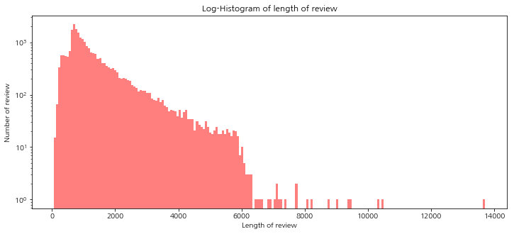
각 리뷰의 문자 길이 분포
train_length = train_data['review'].apply(len)
train_length.head()
0 2302
1 946
2 2449
3 2245
4 2231
Name: review, dtype: int64
plt.figure(figsize=(12,5))
plt.hist(train_length, bins=200, alpha=0.5, color='r', label='word')
plt.yscale('log', nonposy='clip')
plt.title('Log-Histogram of length of review')
plt.xlabel('Length of review')
plt.ylabel('Number of review')
Text(0, 0.5, 'Number of review')
 png
png
- figsize: (가로, 세로) 형태의 튜플로 입력
- bins: 히스토그램 값들에 대한 버켓 범위
- range: x축 값의 범위
- alpha: 그래프 색상 투명도
- color: 그래프 색상
- label: 그래프에 대한 라벨
대부분 6000 이하 그중에서도 2000 이하에 분포되어 있음을 알 수 있다. 그리고 일부 데이터의 경우 이상치로 10000 이상의 값을 가지고 있다.
길이데 대해 몇가지 통계를 확인해 보자
print('리뷰 길이 최대 값: {}'.format(np.max(train_length)))
print('리뷰 길이 최소 값: {}'.format(np.min(train_length)))
print('리뷰 길이 평균 값: {:.2f}'.format(np.mean(train_length)))
print('리뷰 길이 표준편차: {:.2f}'.format(np.std(train_length)))
print('리뷰 길이 중간 값: {}'.format(np.median(train_length)))
# 사분위의 대한 경우는 0~100 스케일로 되어있음
print('리뷰 길이 제 1 사분위: {}'.format(np.percentile(train_length, 25)))
print('리뷰 길이 제 3 사분위: {}'.format(np.percentile(train_length, 75)))
리뷰 길이 최대 값: 13708
리뷰 길이 최소 값: 52
리뷰 길이 평균 값: 1327.71
리뷰 길이 표준편차: 1005.22
리뷰 길이 중간 값: 981.0
리뷰 길이 제 1 사분위: 703.0
리뷰 길이 제 3 사분위: 1617.0
리뷰의 길이가 히스토그램에서 확인했던 것과 비슷하게 평균이 1300정도 이고, 최댓값이 13000이로 확인이 된다.
plt.figure(figsize=(12,5))
plt.boxplot(train_length, labels=['counts'], showmeans=True)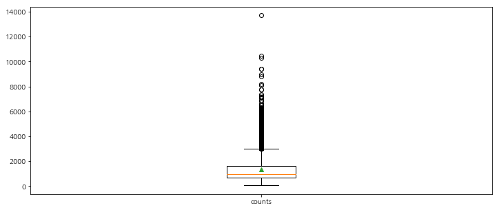 png
png
- labels : 입력한 데이터에 대한 라벨
- showmeans : 평균값을 마크함
데이터의 길이가 대부분 2000 이하로 평균이 1500 이하인데, 길이가 4000 이상인 이상치 데이터도 많이 분포되어 있는 것을 확인할 수 있다.
이제 리뷰에서 많이 사용된 단어로 어떤 것이 있는지 알아보자.
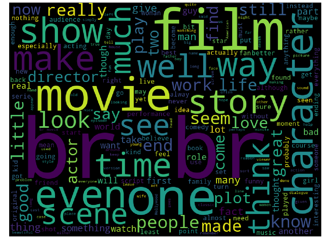
많이 사용된 단어
from wordcloud import WordCloud
cloud = WordCloud(width=800, height=600).generate(" ".join(train_data['review']))
plt.figure(figsize=(20, 15))
plt.imshow(cloud)
plt.axis('off')
(-0.5, 799.5, 599.5, -0.5)
 png
png
워드 클라우드를 통해 살펴보면 가장 많이 사용된 단어는 br로 확인이 된다. br은 HTML 태그 이기때문에 이 태그들을 모두 제거 하는 전처리 작업이 필요하다.
긍정/부정 데이터의 분포
fig, axe = plt.subplots(ncols=1)
fig.set_size_inches(6, 3)
sns.countplot(train_data['sentiment'])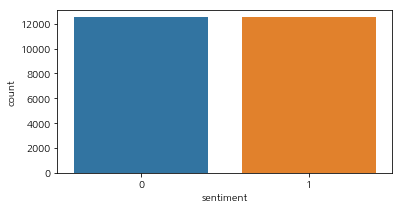 png
png
거의 동일한 개수로 분포되어 있음을 확인할 수 있다. 좀더 정확한 값을 확인해 보자.
print("긍정 리뷰 개수: {}".format(train_data['sentiment'].value_counts()[1]))
print("부정 리뷰 개수: {}".format(train_data['sentiment'].value_counts()[0]))
긍정 리뷰 개수: 12500
부정 리뷰 개수: 12500
각 리뷰의 단어 개수 분포
각 리뷰를 단어 기준으로 나눠서 각 리뷰당 단어의 개수를 확인해 보자.
단어는 띄어쓰기 기준으로 하나의 단어라 생각하고 개수를 계산한다.
우선 각 단어의 길이를 가지는 변수를 하나 설정하자.
train_word_counts = train_data['review'].apply(lambda x:len(x.split(' ')))plt.figure(figsize=(15, 10))
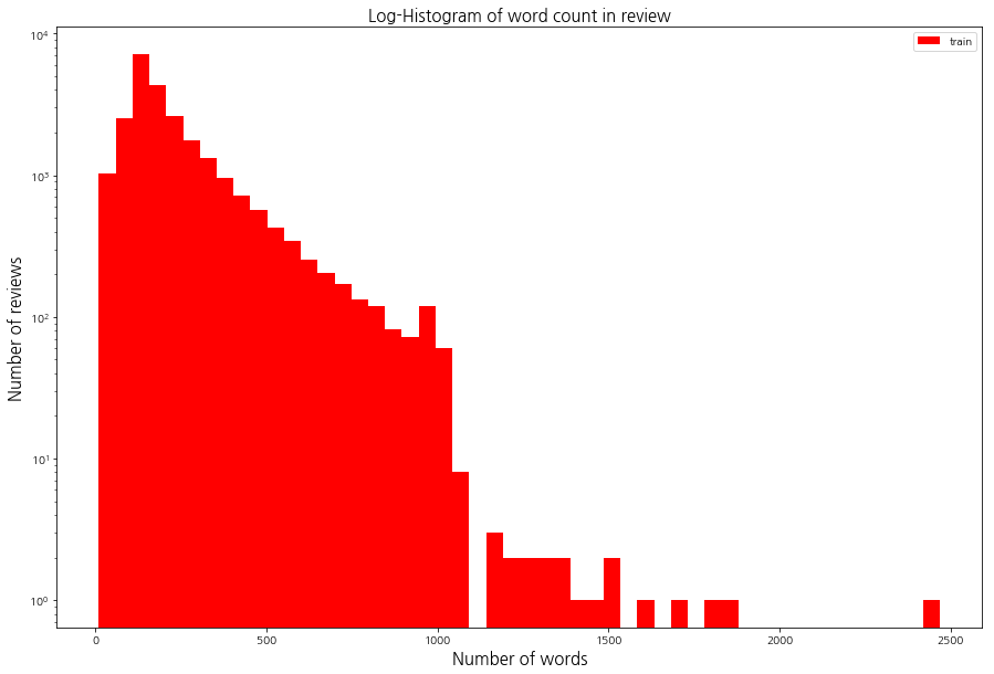
plt.hist(train_word_counts, bins=50, facecolor='r',label='train')
plt.title('Log-Histogram of word count in review', fontsize=15)
plt.yscale('log', nonposy='clip')
plt.legend()
plt.xlabel('Number of words', fontsize=15)
plt.ylabel('Number of reviews', fontsize=15)Text(0, 0.5, 'Number of reviews')
 png
png
대부분의 단어가 1000개 미만의 단어를 가지고 있고, 대부분 200개 정도의 단어를 가지고 있다.
print('리뷰 단어 개수 최대 값: {}'.format(np.max(train_word_counts)))
print('리뷰 단어 개수 최소 값: {}'.format(np.min(train_word_counts)))
print('리뷰 단어 개수 평균 값: {:.2f}'.format(np.mean(train_word_counts)))
print('리뷰 단어 개수 표준편차: {:.2f}'.format(np.std(train_word_counts)))
print('리뷰 단어 개수 중간 값: {}'.format(np.median(train_word_counts)))
# 사분위의 대한 경우는 0~100 스케일로 되어있음
print('리뷰 단어 개수 제 1 사분위: {}'.format(np.percentile(train_word_counts, 25)))
print('리뷰 단어 개수 제 3 사분위: {}'.format(np.percentile(train_word_counts, 75)))
리뷰 단어 개수 최대 값: 2470
리뷰 단어 개수 최소 값: 10
리뷰 단어 개수 평균 값: 233.79
리뷰 단어 개수 표준편차: 173.74
리뷰 단어 개수 중간 값: 174.0
리뷰 단어 개수 제 1 사분위: 127.0
리뷰 단어 개수 제 3 사분위: 284.0
통계를 살펴보면 평균이 233개, 최댓값은 2470개의 단어를 가지고 있다. 그리고 3사분위 값이 284개로 리뷰의 75%가 300개 이하의 단어를 가지고 있음을 확인 할 수 있다.
특수문자 및 대/소문자 비율
qmarks = np.mean(train_data['review'].apply(lambda x: '?' in x)) # 물음표가 구두점으로 쓰임
fullstop = np.mean(train_data['review'].apply(lambda x: '.' in x)) # 마침표
capital_first = np.mean(train_data['review'].apply(lambda x: x[0].isupper())) #  첫번째 대문자
capitals = np.mean(train_data['review'].apply(lambda x: max([y.isupper() for y in x]))) # 대문자가 몇개
numbers = np.mean(train_data['review'].apply(lambda x: max([y.isdigit() for y in x]))) # 숫자가 몇개

print('물음표가있는 질문: {:.2f}%'.format(qmarks * 100))
print('마침표가 있는 질문: {:.2f}%'.format(fullstop * 100))
print('첫 글자가 대문자 인 질문: {:.2f}%'.format(capital_first * 100))
print('대문자가있는 질문: {:.2f}%'.format(capitals * 100))
print('숫자가있는 질문: {:.2f}%'.format(numbers * 100))
물음표가있는 질문: 29.55%
마침표가 있는 질문: 99.69%
첫 글자가 대문자 인 질문: 92.84%
대문자가있는 질문: 99.59%
숫자가있는 질문: 56.66%
결과를 보면 대부분 마침표를 포함하고 있고, 대문자도 대부분 사용하고 있다. 따라서 전처리 과정에서 대문자의 경우 모두 소문자로 바꾸고 특수 문자의 경우 제거해야 한다. 이 과정은 학습에 방해가 되는 요소들을 제거하기 위함이다.
데이터 전처리
import re
import pandas
import numpy
import json
from bs4 import BeautifulSoup
from nltk.corpus import stopwords
from tensorflow.python.keras.preprocessing.sequence import pad_sequences
from tensorflow.python.keras.preprocessing.text import Tokenizer
어떤 방향으로 전처리해야 할지 결정하기 위해 데이터 하나를 자세히 보자.
DATA_IN_PATH = './data_in/'

train_data = pd.read_csv(DATA_IN_PATH + 'labeledTrainData.tsv', header = 0, delimiter = '\t', quoting = 3)
print(train_data['review'][0])
"With all this stuff going down at the moment with MJ...bad m'kay.
...I hope he is not the latter."
우선 <br/>과 같은 HTML 태그와 \,... 같은 특수문자가 포함되어 있는것을 확인할 수 있는데, 이는 일반적으로 문장의 의미에 크게 영향을 주지 않기 때문에 BeautifulSoup과 re.sub을 이용해 제거하자.
review = train_data['review'][0] # 리뷰들중 하나.
review_text = BeautifulSoup(review, "html5lib").get_text() # HTML 태그 제거
review_text = re.sub("[^a-zA-Z]", " ", review_text) # 영어 문자를 제외한 나머지는 모두 공백으로 변경
print(review_text)
With all this stuff going ... I hope he is not the latter
stop_words = set(stopwords.words('english')) # 영어 불용어들의 set을 만듬

review_text = review_text.lower() # 소문자변환 (NLTK에서 제공하는 불용어 사전은 모두 소문자로 되어있다.)
words = review_text.split() # 단어리스트로 변환
words = [w for w in words if not w in stop_words] # 불용어를 제거한 리스트를 만듬
print(words)
['stuff', 'going', 'moment', 'mj', 'started', 'listening',,,'hope', 'latter']
clean_review = ' '.join(words) # 단어 리스트들을 다시 하나의 문장으로 합친다.
print(clean_review)
stuff going moment mj started listening ... iars hope latter
전체 데이터에 적용하기 위해 함수화 하자.
def preprocessing(review, remove_stopwords=False):
    # 불용어 제거는 선택 가능하도록(경우에 따라 불용어 제거가 역호과를 가져올 수 있다.)

    # 1. HTML 태그 제거
    review_text = BeautifulSoup(review, "html5lib").get_text()

    # 2. 영어가 아닌 특수문자들을 공백(" ")으로 바꾸기
    review_text = re.sub("[^a-zA-Z]", " ", review_text)

    # 3. 대문자들을 소문자로 바꾸고 공백단위로 텍스트들 나눠서 리스트로 만든다.
    words = review_text.lower().split()

    if remove_stopwords:
        # 4. 불용어들을 제거

        #영어에 관련된 불용어 불러오기
        stops = set(stopwords.words("english"))
        # 불용어가 아닌 단어들로 이루어진 새로운 리스트 생성
        words = [w for w in words if not w in stops]
        # 5. 단어 리스트를 공백을 넣어서 하나의 글로 합친다.
        clean_review = ' '.join(words)

    else: # 불용어 제거하지 않을 때
        clean_review = ' '.join(words)

    return clean_review
clean_train_reviews = []
for review in train_data['review']:
clean_train_reviews.append(preprocessing(review, remove_stopwords=True))
# 전처리된 데이터 확인
clean_train_reviews[0]'stuff going moment mj started listening ... sickest liars hope latter'
clean_train_df = pd.DataFrame({'review': clean_train_reviews, 'sentiment': train_data['sentiment']})tokenizer = Tokenizer()
tokenizer.fit_on_texts(clean_train_reviews)
text_sequences = tokenizer.texts_to_sequences(clean_train_reviews)위와 같이 하면 각 리뷰가 텍스트가 아닌 인덱스의 벡터로 구성될 것이다.
print(text_sequences[0])[404, 70, 419, 8815, 506, 2456, 115, 54, 873, ,,, ,18688, 18689, 316, 1356]
전체 데이터가 인덱스로 구성됨에 따라 각 인덱스가 어떤 단어를 의미하는지 확인할 수 있어야 하기 때문에 단어 사전이 필요하다.
word_vocab = tokenizer.word_index
print(str(word_vocab)[:100], "...")
print("전체 단어 개수 : ", len(word_vocab) + 1)


{'movie': 1, 'film': 2, 'one': 3, 'like': 4, 'good': 5, 'time': 6, 'even': 7, 'would': 8, 'story': 9 ...
전체 단어 개수 :  74066
총 74,000개 정도의 단어 이다. 단어 사전뿐 아니라 전체 단어의 개수도 이후 모델에서 사용되기 때문에 저장해 둔다.
data_configs = {}

data_configs['vocab'] = word_vocab
data_configs['vocab_size'] = len(word_vocab) + 1
MAX_SEQUENCE_LENGTH = 174 # 문장 최대 길이
train_inputs = pad_sequences(text_sequences, maxlen=MAX_SEQUENCE_LENGTH, padding='post')
print('Shape of train data: ', train_inputs.shape)Shape of train data: (25000, 174)
패딩 처리를 위해 pad_sequences함수를 사용하였다. 최대 길이를 174로 설정한 것은 앞서 단어 개수의 통계를 계산했을 때 나왔던 중간값이다.
보통 평균이 아닌 중간값을 사용하는 경우가 많은데, 일부 이상치 데이터로 인해 평균값이 왜곡될 우려가 있기때문이다.
패딩 처리를 통해 데이터의 형태가 25,000개의 데이터가 174라는 길이를 동일하게 가지게 되었다.
train_labels = np.array(train_data['sentiment'])
print('Shape of label tensor:', train_labels.shape)
Shape of label tensor: (25000,)
numpy 배열로 만든 후 라벨의 형태를 확인해 보면 길이가 25,000인 벡터임을 확인할 수 있다.
이렇게 라벨까지 numpy 배열로 저장하면 모든 전처리 과정이 끝난다.
원본 데이터를 벡터화하는 과정을 그림을 통해 이해해 보자.
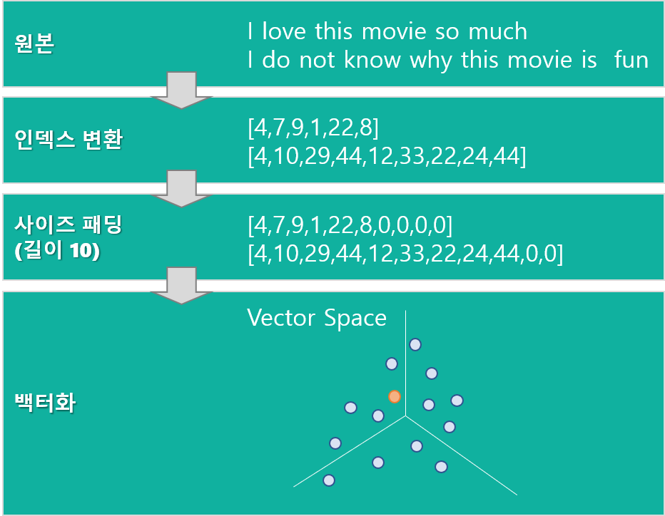 oorigin-vector
이제 전처리한 데이터를 이후 모델링 과정에서 사용하기 위해 저장을 하도록 하자.
TRAIN_INPUT_DATA = 'train_input.npy'
TRAIN_LABEL_DATA = 'train_label.npy'
TRAIN_CLEAN_DATA = 'train_clean.csv'
DATA_CONFIGS = 'data_configs.json'

import os
# 저장하는 디렉토리가 존재하지 않으면 생성
if not os.path.exists(DATA_IN_PATH):
    os.makedirs(DATA_IN_PATH)


# 전처리 된 데이터를 넘파이 형태로 저장
np.save(open(DATA_IN_PATH + TRAIN_INPUT_DATA, 'wb'), train_inputs)
np.save(open(DATA_IN_PATH + TRAIN_LABEL_DATA, 'wb'), train_labels)

# 정제된 텍스트를 csv 형태로 저장
clean_train_df.to_csv(DATA_IN_PATH + TRAIN_CLEAN_DATA, index = False)


# 데이터 사전을 json 형태로 저장
json.dump(data_configs, open(DATA_IN_PATH + DATA_CONFIGS, 'w'), ensure_ascii=False)
test 데이터도 동일하게 저장하자. 다만 test 데이터는 라벨 값이 없기 때문에 라벨은 따로 저장하지 않아도 된다. 추가로 test 데이터네 대해 저장해야 하는 값이 있는데 각 리뷰 데이터에 대해 리뷰에 대한 id값을 저장해야 한다.
test_data = pd.read_csv(DATA_IN_PATH + "testData.tsv", header=0, delimiter="\t", quoting=3)

clean_test_reviews = []
for review in test_data['review']:
    clean_test_reviews.append(preprocessing(review, remove_stopwords = True))


clean_test_df = pd.DataFrame({'review': clean_test_reviews, 'id': test_data['id']})
test_id = np.array(test_data['id'])

text_sequences = tokenizer.texts_to_sequences(clean_test_reviews)
test_inputs = pad_sequences(text_sequences, maxlen=MAX_SEQUENCE_LENGTH, padding='post')


TEST_INPUT_DATA = 'test_input.npy'
TEST_CLEAN_DATA = 'test_clean.csv'
TEST_ID_DATA = 'test_id.npy'

np.save(open(DATA_IN_PATH + TEST_INPUT_DATA, 'wb'), test_inputs)
np.save(open(DATA_IN_PATH + TEST_ID_DATA, 'wb'), test_id)
clean_test_df.to_csv(DATA_IN_PATH + TEST_CLEAN_DATA, index = False)
test 데이터를 전처리할 떄 한 가지 중요한 점은 토크나이저를 통해 인덱스 벡터로 만들 때 토크나이징 객체로 새롭게 만드는 것이 아니라, 기존에 학습 데이터에 적용한 토크나이저 객체를 사용해야 한다는 것이다. 만약 새롭게 만들 경우 Train 데이터와 Test 데이터에 대한 각 단어들의 인덱스가 달라져서 모델에 정상적으로 적용할 수 없기 때문이다.
지금까지의 결과를 아래와 같은 파일들에 각각 저장을 하였다.
단어 인덱스 사전 및 개수 : data_configs.json
훈련 데이터 : train_input.npy, train_label.npy, train_clean.csv
테스트 데이터 : test_input.npy, test_clean.csv, test_id.npy
이제 저장된 데이터를 이용해 다음 스탭을 진행하도록 하겠다.